Effective and Continuous ML

“The most powerful tool we have as developers is automation.” ~ Scott Hanselman

Synopsis

If you have ever worked with ML pipelines of any kind and wondered if it would be possible to combine the training and model saving parts of it with a CI/CD pipeline, 🐳, look no further as it possible and you will learn about it here. The aim of this tutorial is to show you a step-by-step process for creating reproducible pipelines to gather, clean, train, evaluate, and track machine learning models with DVC (data version control), CML (continuous machine learning), and other tools in the Data Science stack. By the end of this tutorial, you will have the tools to create your own reproducible pipelines and experiment with different tools and models to heart’s content.

Learning Outcomes

By the end of the tutorial you would have learned

1. a bit of git for keeping track of your code
2. a bit of dvc to track your different datasets and machine learning models
3. a bit of CI/CD pipelines with CML
4. a bit of ML and some python tools for it

Table of Contents

1. Scenario
2. The Tools
3. Environment Set Up
4. The Data
   • Getting the Data
   • Preparing the Data
5. Training our First Model
6. Model Evaluation
7. DVC Pipelines
8. CI/CD Pipelines with CML
9. Experiments
10. Merging our Changes - PRs
11. Summary
12. Blind Spots and Future Work
13. Resources

NB: this tutorial was built in a Linux machine and some terminal commands might only be available in *NIX-based systems.

1. Scenario

Imagine you work at a data analytics consultancy called XYZ Analytics, and that your boss comes to you with a new challenge for you, to create a machine learning model to predict the amount of bikes neeeded at any given hour of the day in Seoul, South Korea. You don’t know anything about bicycle rental systems but you’re excited to take on the challenge and accept it with pleasure.

The challenge was presented to your boss by the South Korean government, and what they are hoping to get later on is an in-house analytical product that anyone can use to figure out the amount of rental bicycles needed at any given time and at different locations in the city of Seoul. You will tackle the predictive modeling part while the rest of team will work on the application and the geospatial part of the task.

Lastly, XYZ Analytics has been improving their data science capabilities and would like for every project to use data and model version control tools, which means you will be using dvc and other cool tools for the first time for this task. Let’s go over the tooling in the next section.

2. The Tools

Here are some of the tools that us, data scientists, might not have much experience with.

• DVC - “Data Version Control, or DVC, is a data and ML experiment management tool that takes advantage of the existing engineering toolset that you’re already familiar with (Git, CI/CD, etc.).”
• CML - “is an open-source library for implementing continuous integration & delivery (CI/CD) in machine learning projects. Use it to automate parts of your development workflow, including model training and evaluation, comparing ML experiments across your project history, and monitoring changing datasets.”
• GitHub Actions - “GitHub Actions help you automate tasks within your software development life cycle. GitHub Actions are event-driven, meaning that you can run a series of commands after a specified event has occurred.”

The rest of the tools we will be using, which should be more familiar to data scientists, are the following ones.

• NumPy - “It is a Python library that provides a multidimensional array object, various derived objects (such as masked arrays and matrices), and an assortment of routines for fast operations on arrays, including mathematical, logical, shape manipulation, sorting, selecting, I/O, discrete Fourier transforms, basic linear algebra, basic statistical operations, random simulation and much more.”
• pandas - “is a fast, powerful, flexible and easy to use open source data analysis and manipulation tool, built on top of the Python programming language.”
• scikit-learn - “is an open source machine learning library that supports supervised and unsupervised learning. It also provides various tools for model fitting, data preprocessing, model selection and evaluation, and many other utilities.”
• XGBoost - “is an optimized distributed gradient boosting library designed to be highly efficient, flexible and portable. It implements machine learning algorithms under the Gradient Boosting framework. XGBoost provides a parallel tree boosting (also known as GBDT, GBM) that solve many data science problems in a fast and accurate way.”
• LightGBM - “is a gradient boosting framework that uses tree based learning algorithms. It is designed to be distributed and efficient with the following advantages: Faster training speed and higher efficiency, lower memory usage, better accuracy, support of parallel, distributed, and GPU learning, and capable of handling large-scale data.”
• CatBoost - “CatBoost is a machine learning algorithm that uses gradient boosting on decision trees. It is available as an open source library.”
• Jupyter Lab - “is a web-based interactive development environment for Jupyter notebooks, code, and data.”
• Git - “Git is a free and open source distributed version control system designed to handle everything from small to very large projects with speed and efficiency.”

Let’s now set up our development environment and get started with our project.

NB: the definitions above have been taken directly from their respective websites.

3. Environment Set Up

The first thing we’ll do is to set up our development environment. We want to make sure the code we develop is reproducible by anyone, anywhere, and without any difficulties. We will use conda here but feel free to use virtualenv, pipenv, or any other environment generating tool you prefer. Open up a terminal, and follow the steps below.

# create the project directory and switch to it
mkdir bikes_ml
cd bikes_ml

# create your env and activate it
conda create -n bikes_ml python=3.9 pip jupyterlab -y
conda activate bikes_ml

# install the tools we will be using
pip install pandas numpy scikit-learn xgboost lightgbm catboost "dvc[s3]"

Note that we did not install most of the packages we’ll use while creating the environment because the installation guide for some of these libraries suggested that we use pip instead of conda.

Our next step is to create a few of the directories we’ll need for the project and a README.md file. The result would look like this.

.
├── data
│   ├── processed
│   │   ├── test
│   │   └── train
│   └── raw
├── metrics
├── models
├── notebooks
├── src
└── README.md

mkdir -p models src notebooks data/processed data/raw metrics .github/workflows
touch README.md

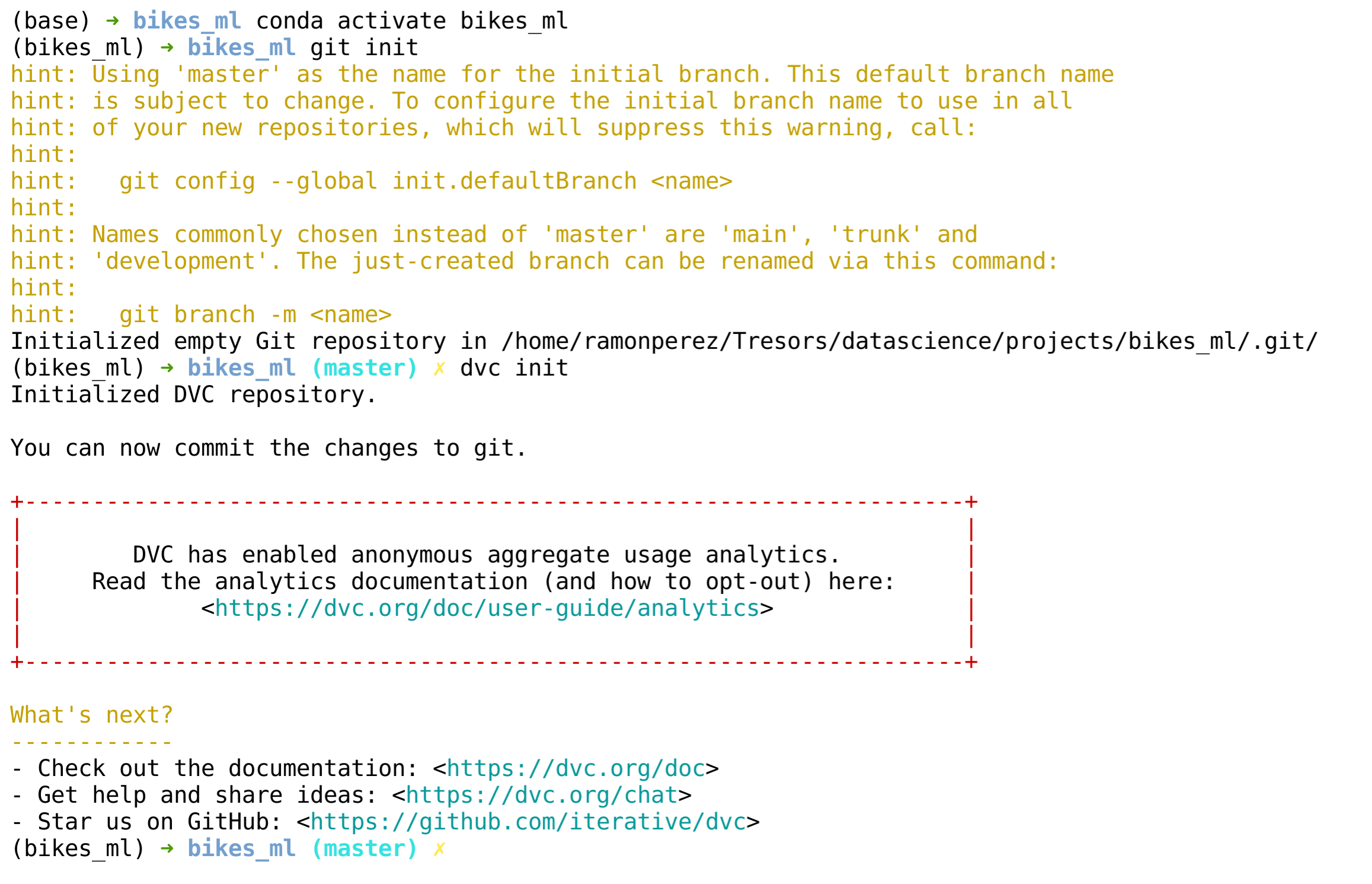
Let’s now initialize our git and dvc repository with the following commands.

git init

dvc init

You should see the following output.

Now that we have everything we need, we can open up our IDE using the jupyter lab command in the terminal. (You should see the following output minus the README.md file.)

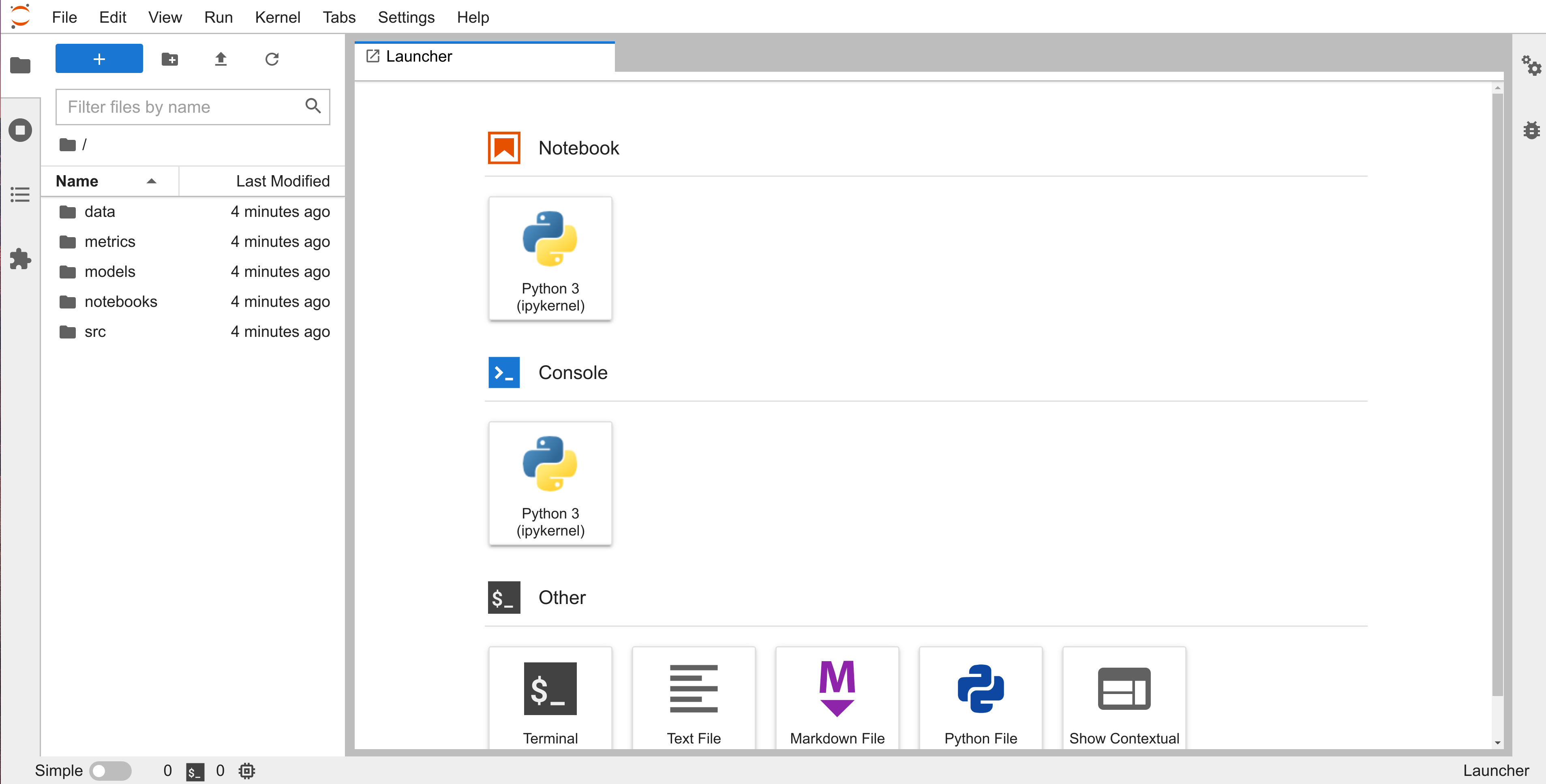
After you open Jupyter Lab, create a notebook in the notebooks directory and call it exploration.ipynb. The rest of the tutorial can, and will be, done through the jupyter notebook we just created. Let’s dive in.

NB: You can get conda through the miniconda distribution here.

4. The Data

Following the described scenario above, the data was donated to the UCI ML Repository on 2020-03-01 for a regression task. It contains information regarding the amount of bikes available per hour between 2017 and 2018.

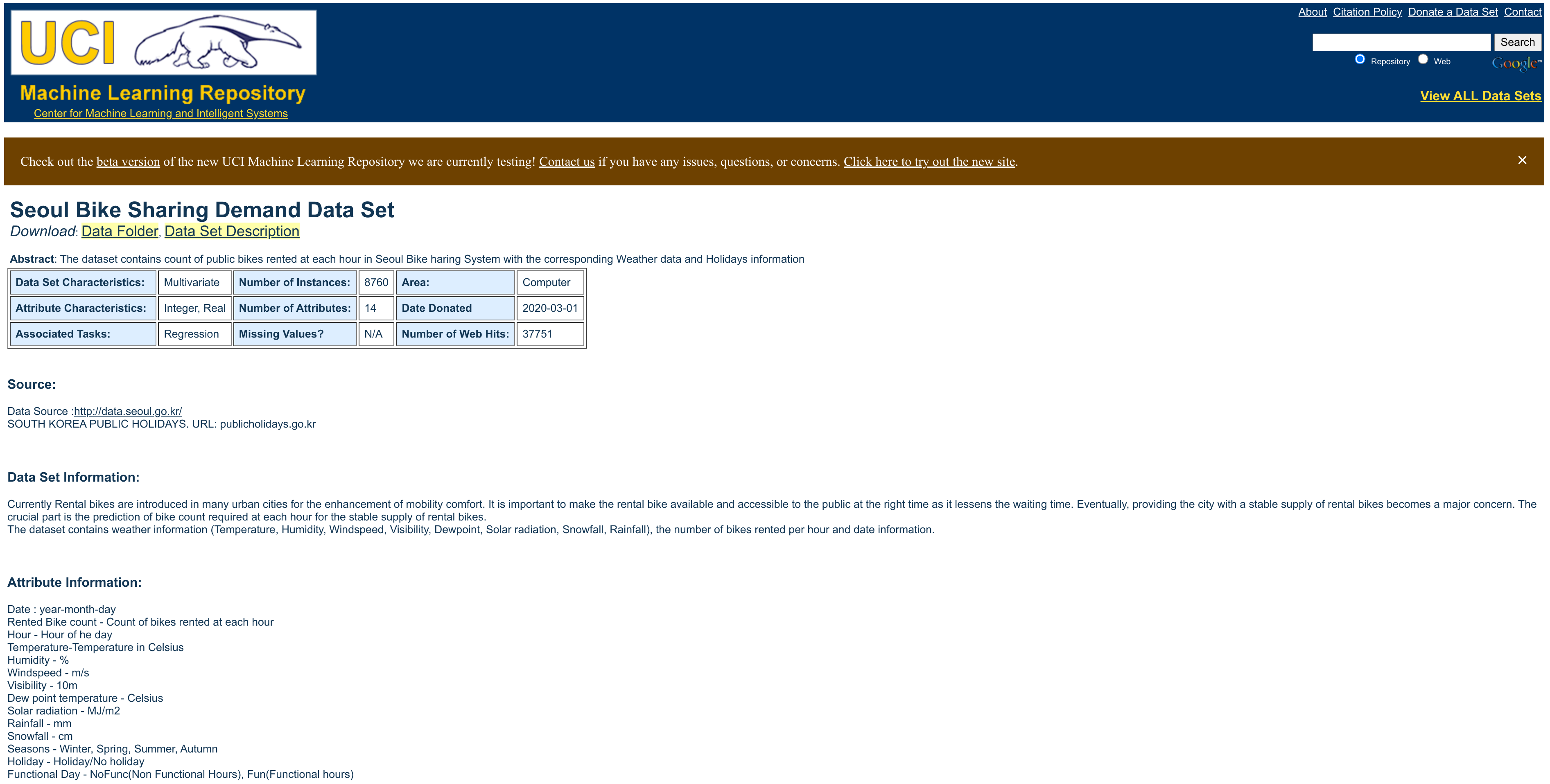
Here are the variables found in the dataset.

• Date - year-month-day
• Rented Bike count - Count of bikes rented at each hour
• Hour - Hour of the day
• Temperature-Temperature in Celsius
• Humidity - %
• Windspeed - m/s
• Visibility - 10m
• Dew point temperature - Celsius
• Solar radiation - MJ/m2
• Rainfall - mm
• Snowfall - cm
• Seasons - Winter, Spring, Summer, and Autumn
• Holiday - Holiday and No holiday
• Functional Day - NoFunc (Non Functional Hours), Fun (Functional hours)

4.1 Getting the Data

We will use the urllib.request and the os libraries to download the data and set up our desired path for it, respectively.

import urllib.request, os

Since we will be running git and dvc commands in the cells below, we need to move up one directory from the notebooks to the root or our project using os.chdir('..') once (and only once).

!pwd

os.chdir('..')

!pwd

The dataset can be downloaded from the URL below and we will give it the filename, SeoulBikeData.csv.

url = 'https://archive.ics.uci.edu/ml/machine-learning-databases/00560/SeoulBikeData.csv'
path_and_filename = os.path.join('data', 'raw', 'SeoulBikeData.csv')

urllib.request.urlretrieve(url, path_and_filename)

Because we want to be able to create a pipeline later on, we will export the few lines of code above as a python script called get_data.py for later use. We will put every python script we want in our pipeline inside the src directory. Get used to this pattern. :)

Also, it is good practice to make sure the directories we are using always exist, so we will add an additional if-else statement to search and/or create it if it does not exist.

The command %%writefile below is a magic function and these are special function of ipython interpreter. The one we are using allows us to write anything in that cell to a file. Others like the %%bash, as we will soon see, make the entire cell a bash executable cell.

%%writefile src/get_data.py

import urllib.request, os

url = 'https://archive.ics.uci.edu/ml/machine-learning-databases/00560/SeoulBikeData.csv'
path = os.path.join('data', 'raw')
filename = 'SeoulBikeData.csv'

if not os.path.exists(path): os.makedirs(path)

urllib.request.urlretrieve(url, os.path.join(path, filename))

Now that we have our dataset, let’s go ahead and add it to our remote storage and start keeping track of the changes that we make to it with dvc. We will use s3 as our primary storage tool for the tutorial but feel free to use the option that best suits your needs and experience from the dvc website. Here are the step to do it with AWS.

1. Log into your AWS account
2. Navigate to Identity and Access Management (IAM) > Access Management > Users
3. Click on Add users
4. Add a name under Set user details, e.g. bikes
5. In the Select AWS access type, check the box [x] next to Access key - Programmatic access
6. In the Set permissions section, click on Attach existing policies directly and search and select AmazonS3FullAccess
7. Accept the rest of the defaults, create your user and download the csv file with your Access key ID and your Secret access key
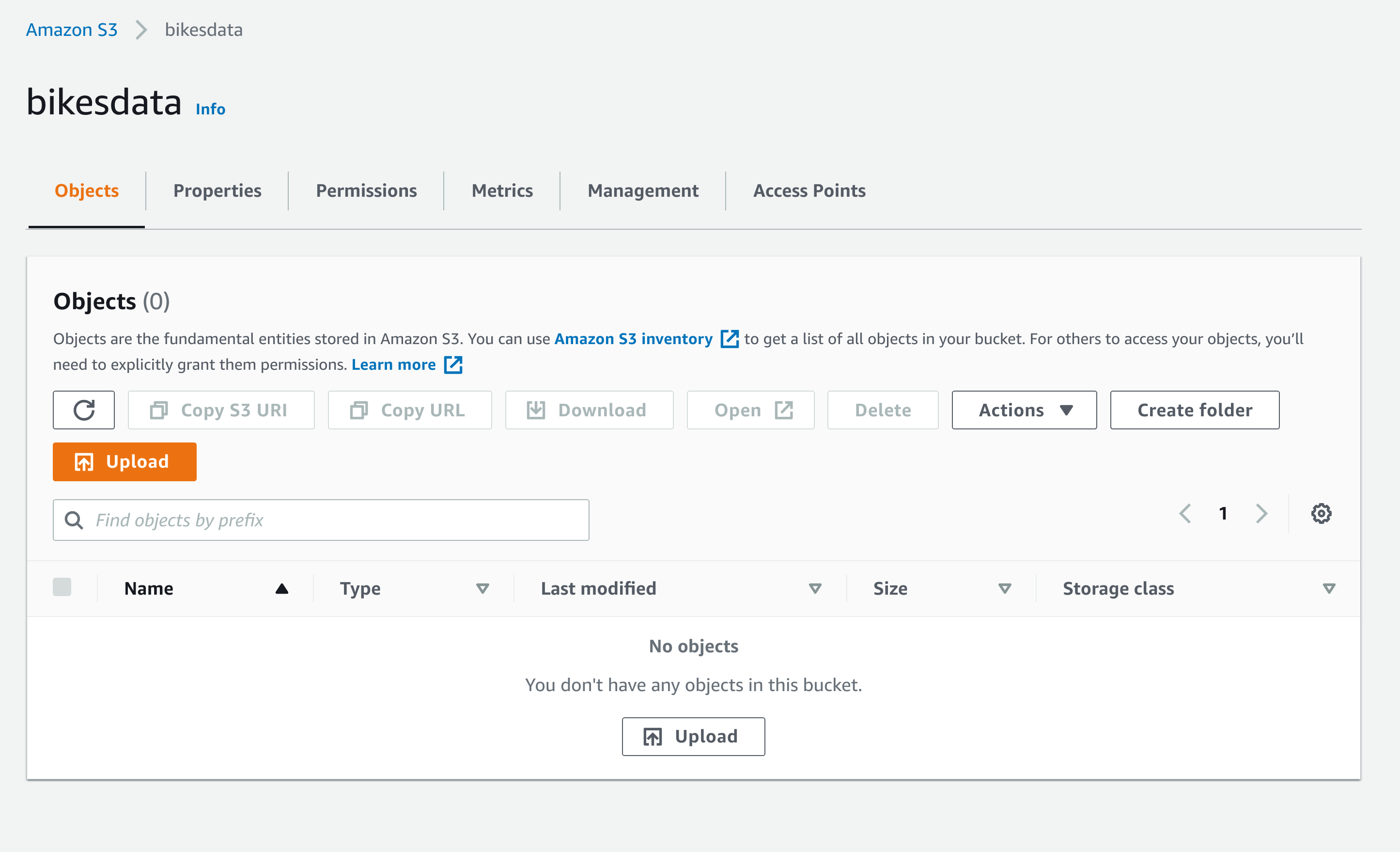
8. Navigate to the S3 Management Console and create a new bucket with the default settings, mine is bikesdata
9. Navigate to your bucket’s Permissions tab and in the Bucket policy section click on Edit and the click on Policy generator
   • In the Select Type of Policy select S3 Bucket Policy
   • In the Principal box add your user’s arn code, e.g. arn:aws:iam::123456789135:user/bikes
   • In the Actions box, select ListBucket
   • In the Amazon Resource Name add your bucket’s arn, e.g. arn:aws:s3:::bikesdata
   • Click on Add Statement
   • Click on Generate Policy and then copy Policy JSON Document
   • Add the policy to your bucket and save the changes

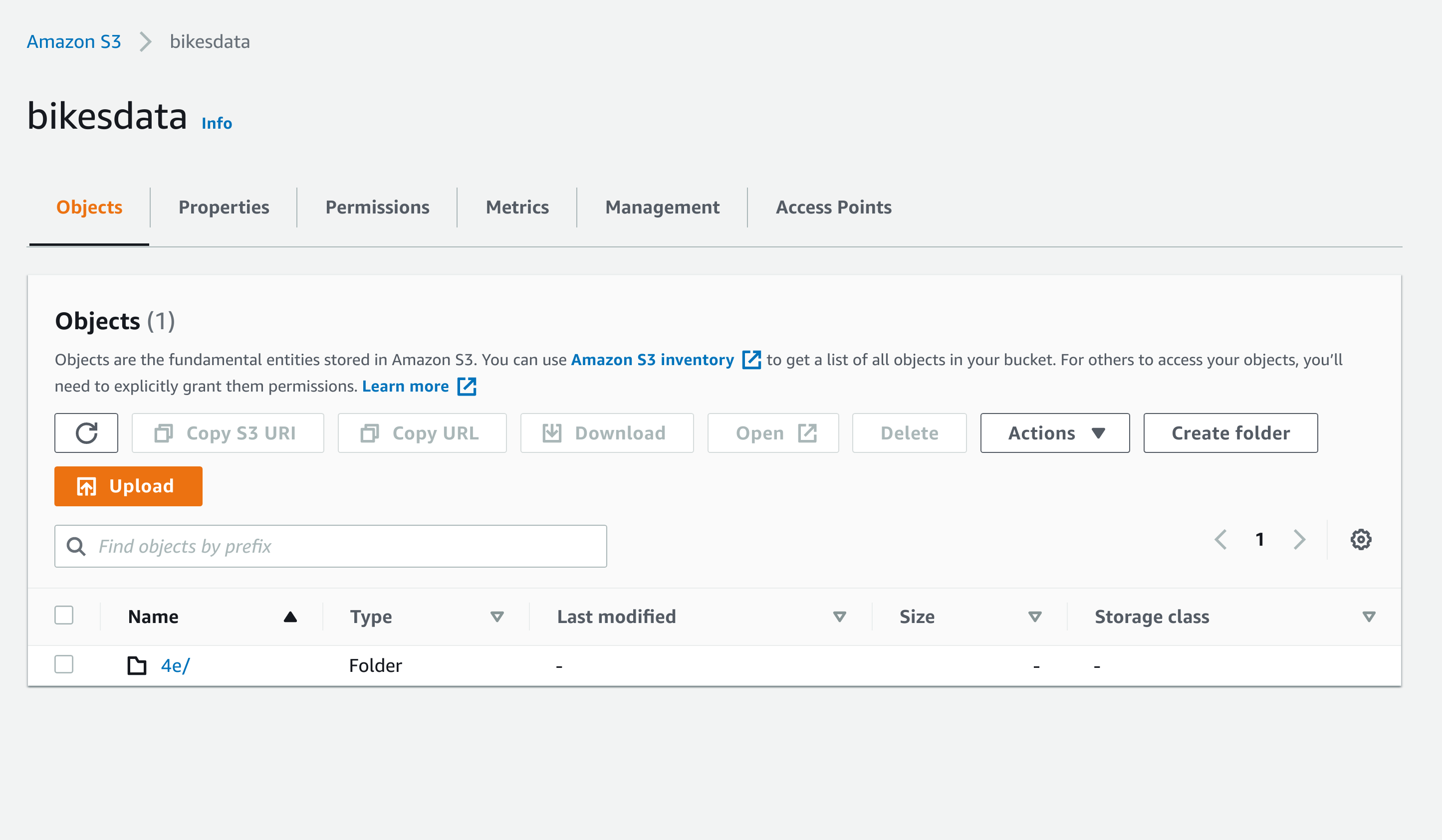
Our Bucket without the data should look as follows.

Now let’s add our bucket to our dvc repo.

%%bash

dvc remote add -d bikestorage s3://bikesdata
dvc remote modify --local bikestorage access_key_id 'AKIAZ2HP4H7DV6XSBGWV'
dvc remote modify --local bikestorage secret_access_key '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'
dvc remote modify bikestorage listobjects true

In the first line above the -d stands for default and bikestorage is the name we have decided on for our bucket. The last piece is the url that directs dvc to our s3 bucket. You can find out more about the remote command through the official docummentation here.

In the next few lines, where we use the modify command to update our dvc local files, we give dvc the resources necessary to access our remote storage from our local computer. If you were to have the awscli installed and configured in your machine, you could have skipped the modify parts of the above cell. You can find more about the modify command through the official docummentation here

Make sure to always keep your credentials in a safe and secure place.

Now let’s start tracking our data and make sure our remote storage is fully connected to our local storage.

%%bash

dvc add data/raw/SeoulBikeData.csv
dvc push

DVC uses special names to keep track of files, so there’s no need to try and figure out what the above name means. Everything in our bucket can always be accessed through dvc.

Lastly, we’ll commit our changes to our git repo after making sure we add the two files created by dvc, data/raw/.gitignore and data/raw/SeoulBikeData.csv.dvc. What dvc is doing is tracking some information about our dataset through git, hence the files ...Data.csv.dvc and .gitignore with the actual data file, while the actual data goes to our remote storage.

%%bash

git add data/raw/.gitignore data/raw/SeoulBikeData.csv.dvc
git commit -m "Start Tracking Data"

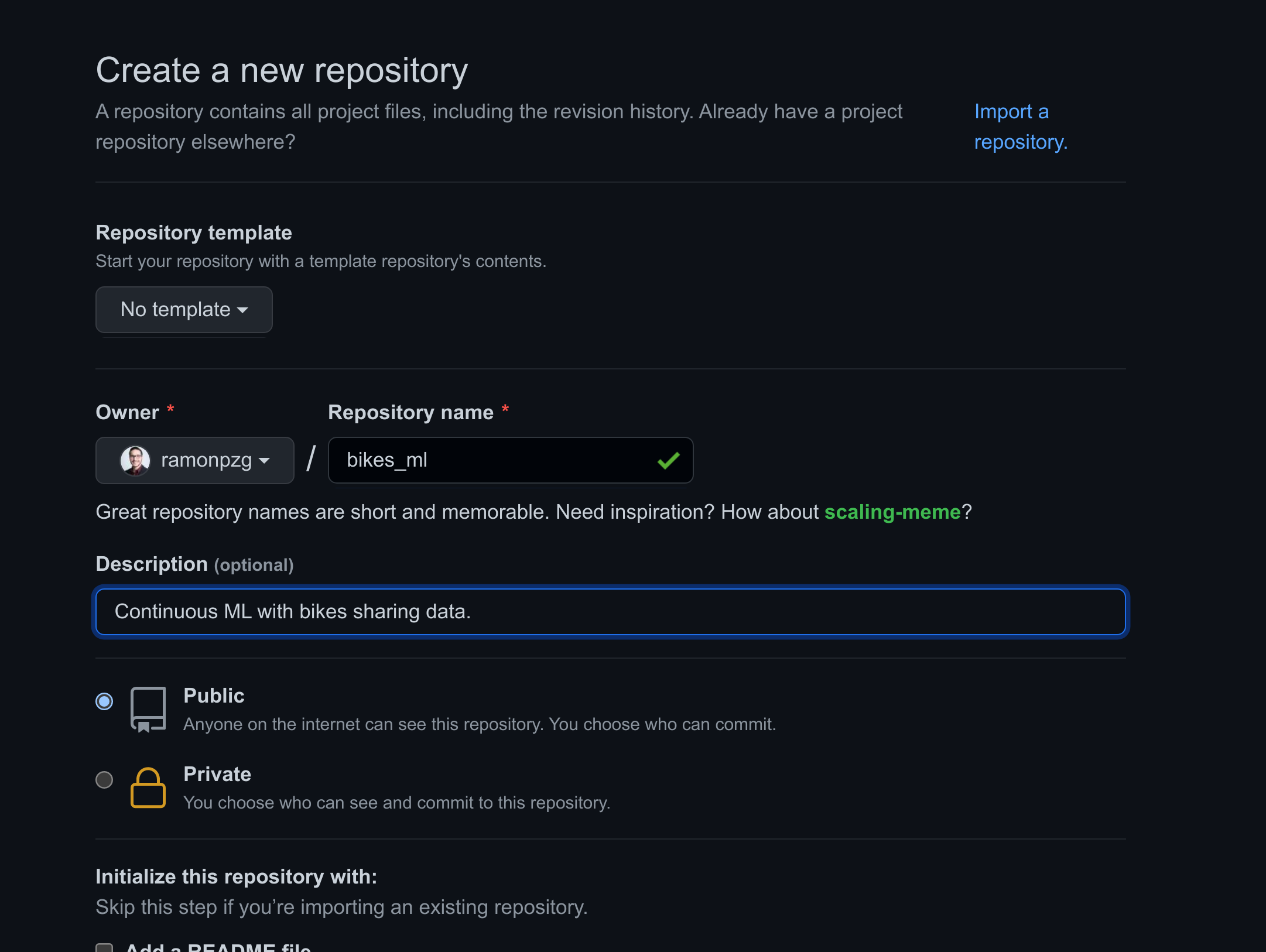
Before we push any changes to GitHub, make sure you create your repository, as shown below, and then connect your local and remote repo with the commands below.

%%bash

git remote add origin https://github.com/ramonpzg/bikes_ml.git
git push -u origin master

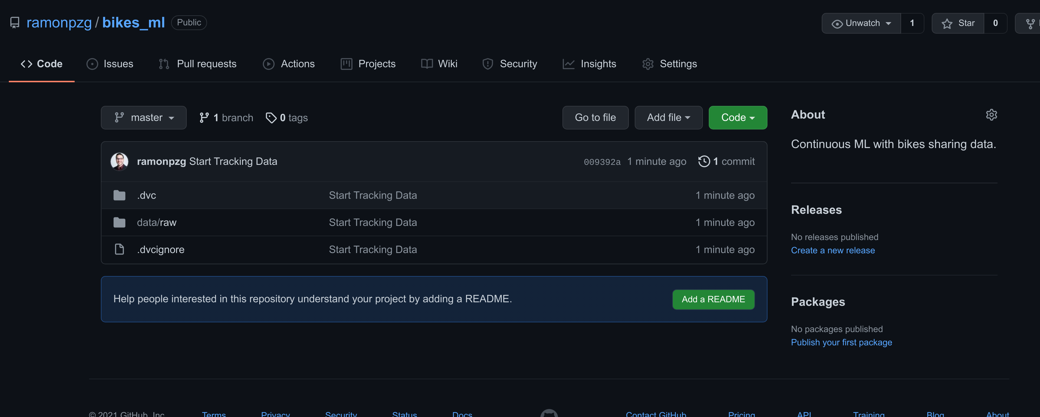
After pushing the changes to GitHub you should see the files in the image below.

4.2 Preparing the Data

The following steps should feel familiar to us, we want to separate the date variable into its components, create dummy variables for the categorical features, normalize the columns so that they only contain alphanumerical characters with underscores instead of spaces, and finally split the data into train and test sets.

import pandas as pd

data = pd.read_csv('data/raw/SeoulBikeData.csv', encoding='iso-8859-1')
data.head()

	Date	Rented Bike Count	Hour	Temperature(°C)	Humidity(%)	Wind speed (m/s)	Visibility (10m)	Dew point temperature(°C)	Solar Radiation (MJ/m2)	Rainfall(mm)	Snowfall (cm)	Seasons	Holiday	Functioning Day
0	01/12/2017	254	0	-5.2	37	2.2	2000	-17.6	0.0	0.0	0.0	Winter	No Holiday	Yes
1	01/12/2017	204	1	-5.5	38	0.8	2000	-17.6	0.0	0.0	0.0	Winter	No Holiday	Yes
2	01/12/2017	173	2	-6.0	39	1.0	2000	-17.7	0.0	0.0	0.0	Winter	No Holiday	Yes
3	01/12/2017	107	3	-6.2	40	0.9	2000	-17.6	0.0	0.0	0.0	Winter	No Holiday	Yes
4	01/12/2017	78	4	-6.0	36	2.3	2000	-18.6	0.0	0.0	0.0	Winter	No Holiday	Yes

data['Date'] = pd.to_datetime(data['Date'])

data.sort_values(['Date', 'Hour'], inplace=True)
data["Year"] = data['Date'].dt.year
data["Month"] = data['Date'].dt.month
data["Week"] = data['Date'].dt.isocalendar().week
data["Day"] = data['Date'].dt.day
data["Dayofweek"] = data['Date'].dt.dayofweek
data["Dayofyear"] = data['Date'].dt.dayofyear
data["Is_month_end"] = data['Date'].dt.is_month_end
data["Is_month_start"] = data['Date'].dt.is_month_start
data["Is_quarter_end"] = data['Date'].dt.is_quarter_end
data["Is_quarter_start"] = data['Date'].dt.is_quarter_start
data["Is_year_end"] = data['Date'].dt.is_year_end
data["Is_year_start"] = data['Date'].dt.is_year_start
data.drop('Date', axis=1, inplace=True)

data = pd.get_dummies(data=data, columns=['Holiday', 'Seasons', 'Functioning Day'])

data.columns = ['rented_bike_count', 'hour', 'temperature', 'humidity', 'wind_speed', 'visibility', 
                'dew_point_temperature', 'solar_radiation', 'rainfall', 'snowfall', 'year', 
                'month', 'week', 'day', 'dayofweek', 'dayofyear', 'is_month_end', 'is_month_start',
                'is_quarter_end', 'is_quarter_start', 'is_year_end', 'is_year_start',
                'seasons_autumn', 'seasons_winter', 'seasons_summer', 'seasons_spring',
                'holiday_yes', 'holiday_no', 'functioning_day_no', 'functioning_day_yes']

split = 0.30
n_train = int(len(data) - len(data) * split)

train_path = os.path.join('data', 'processed', 'train.csv')
test_path = os.path.join('data', 'processed', 'test.csv')

data[:n_train].reset_index(drop=True).to_csv(train_path, index=False)
data[n_train:].reset_index(drop=True).to_csv(test_path, index=False)

Using the same commands as before, let’s keep track of our new dataset with dvc and push the changes to our s3 bucket. In addition, we’ll create a file called prepared.py for later use in our pipelines.

%%bash

dvc add data/processed/train.csv data/processed/test.csv
dvc push

%%writefile src/prepare.py

import pandas as pd
import os, sys

split = 0.30

raw_data_path = sys.argv[1]
train_path = os.path.join('data', 'processed', 'train.csv')
test_path = os.path.join('data', 'processed', 'test.csv')

# read the data
data = pd.read_csv(raw_data_path, encoding='iso-8859-1')

# add date vars
data['Date'] = pd.to_datetime(data['Date'])
data.sort_values(['Date', 'Hour'], inplace=True)
data["Year"] = data['Date'].dt.year
data["Month"] = data['Date'].dt.month
data["Week"] = data['Date'].dt.isocalendar().week
data["Day"] = data['Date'].dt.day
data["Dayofweek"] = data['Date'].dt.dayofweek
data["Dayofyear"] = data['Date'].dt.dayofyear
data["Is_month_end"] = data['Date'].dt.is_month_end
data["Is_month_start"] = data['Date'].dt.is_month_start
data["Is_quarter_end"] = data['Date'].dt.is_quarter_end
data["Is_quarter_start"] = data['Date'].dt.is_quarter_start
data["Is_year_end"] = data['Date'].dt.is_year_end
data["Is_year_start"] = data['Date'].dt.is_year_start
data.drop('Date', axis=1, inplace=True)

# add dummies
data = pd.get_dummies(data=data, columns=['Holiday', 'Seasons', 'Functioning Day'])

# Normalize columns
data.columns = ['rented_bike_count', 'hour', 'temperature', 'humidity', 'wind_speed', 'visibility', 
                'dew_point_temperature', 'solar_radiation', 'rainfall', 'snowfall', 'year', 
                'month', 'week', 'day', 'dayofweek', 'dayofyear', 'is_month_end', 'is_month_start',
                'is_quarter_end', 'is_quarter_start', 'is_year_end', 'is_year_start',
                'seasons_autumn', 'seasons_winter', 'seasons_summer', 'seasons_spring',
                'holiday_yes', 'holiday_no', 'functioning_day_no', 'functioning_day_yes']

n_train = int(len(data) - len(data) * split)
data[:n_train].reset_index(drop=True).to_csv(train_path, index=False)
data[n_train:].reset_index(drop=True).to_csv(test_path, index=False)

Instead of adding file by file with git, it would be better if we were able to use git add . everytime and not worry about commiting something we don’t want to GitHub (e.g. our data). So let’s create a .gitignore file in our project directory, and let’s add a few of the files we don’t want to commit.

%%writefile .gitignore

.ipynb_checkpoints
new_user_credentials.csv

%%bash

git add .
git commit -m "Preparation stage completed"
git push

5. Training our First Model

We want to create a model that predicts how many bikes will be needed at any given hour and on any given date in the future in the city of Seoul. Since the number of bicycles available for rent is a continuous number, this is a regression problem and what a better tool to use for regression problems that Random Forests.

What are Random Forests anyways?

“Random forests or random decision forests are an ensemble learning method for classification, regression and other tasks that operates by constructing a multitude of decision trees at training time. For classification tasks, the output of the random forest is the class selected by most trees. For regression tasks, the mean or average prediction of the individual trees is returned. Random decision forests correct for decision trees’ habit of overfitting to their training set.” ~ Wikipedia

We want to start with a baseline model, evaluate it, and then fine tune either the implementation that we picked, in this case the scikit-learn’s one or, as we’ll see in a later section, an implementation from another framework.

After we train our sklearn model, we want to serialize (or pickle) that model, track it with dvc, and use it later with unseen data in the evaluation stage.

We’ll import sklearn’s RandomForestRegressor and python’s pickle module, load our train set, and start our training with 100 estimators and seed. Feel free to change these however you’d like tho.

from sklearn.ensemble import RandomForestRegressor
import pickle

X_train = pd.read_csv('data/processed/train.csv')
y_train = X_train.pop('rented_bike_count')

seed = 42
n_est = 100

rf = RandomForestRegressor(n_estimators=n_est, random_state=seed)
rf.fit(X_train.values, y_train.values)

rf.predict(X_train.values)[:10]

with open('models/rf_model.pkl', "wb") as fd:
    pickle.dump(rf, fd)

Now that we have a trained model, let’s save the steps we just took to a file called train.py, and let’s also start tracking our model in the same way in which we tracked our data earlier with dvc. Lastly, we’ll commit our work and push everything to GitHub.

%%writefile src/train.py

import os, pickle, sys
import numpy as np, pandas as pd
from sklearn.ensemble import RandomForestRegressor

input_data = sys.argv[1]
output = os.path.join('models', 'rf_model.pkl')
seed = 42
n_est = 100

X_train = pd.read_csv(input_data)
y_train = X_train.pop('rented_bike_count')

rf = RandomForestRegressor(n_estimators=n_est, random_state=seed)
rf.fit(X_train.values, y_train.values)

with open(output, "wb") as fd:
    pickle.dump(rf, fd)

%%bash

dvc add models/rf_model.pkl
dvc push

%%bash

git add .
git commit -m "Training stage completed"
git push

6. Model Evaluation

Model evaluation is a crucial part of training ML models, and it is important that we pick useful metrics that can indicate to us how well our model is perfoming, or expecting to perform, when presented with unseen data.

The metrics we’ll use are Mean Absolute Error, Root Mean Squared Error, and $R^2$.

• Mean Absolute Error - “is a measure of errors between paired observations expressing the same phenomenon. Examples of Y versus X include comparisons of predicted versus observed, subsequent time versus initial time, and one technique of measurement versus an alternative technique of measurement.” ~ Wikipedia
• Root Mean Squared Error - “is a frequently used measure of the differences between values (sample or population values) predicted by a model or an estimator and the values observed. The RMSD serves to aggregate the magnitudes of the errors in predictions for various data points into a single measure of predictive power. RMSD is a measure of accuracy, to compare forecasting errors of different models for a particular dataset and not between datasets, as it is scale-dependent.” ~ Wikipedia
• $R^2$ - “In statistics, the coefficient of determination, also spelt coëfficient, denoted $R^2$ or r2 and pronounced “R squared”, is the proportion of the variation in the dependent variable that is predictable from the independent variable(s).” ~ Wikipedia

We’ll start by loading our model and our test set, predict the test set and compare such predictions with the ground truth. After we compute the metrics above, we want to save them to a JSON file for further use and comparison using dvc.

import sklearn.metrics as metrics, json, numpy as np

with open('models/rf_model.pkl', "rb") as fd:
    model = pickle.load(fd)

X_test = pd.read_csv('data/processed/test.csv')
y_test = X_test.pop('rented_bike_count')

predictions = model.predict(X_test)
predictions[:10]

mae = metrics.mean_absolute_error(y_test.values, predictions)
rmse = np.sqrt(metrics.mean_squared_error(y_test.values, predictions))
r2_score = model.score(X_test.values, y_test.values)

print(f"Mean Absolute Error: {mae:.2f}")
print(f"Root Mean Square Error: {rmse:.2f}")
print(f"R^2: {r2_score:.3f}")

with open(os.path.join('metrics', 'metrics.json'), "w") as fd:
    json.dump({"MAE": mae, "RMSE": rmse, "R^2":r2_score}, fd, indent=4)

We will save the steps above to a file called evaluate.py for futher use later, and we will add our metrics to git and GitHub rather than to our remote s3 bucket. The reason beign that dvc has a special function that allows us to compare the diff of metrics between those in a branch and those in master, and as you’ll see soon, this is a very powerful feature of dvc that we certainly want to take advantage of.

%%writefile src/evaluate.py

import json, os, pickle, sys, pandas as pd, numpy as np
import sklearn.metrics as metrics

model_file = sys.argv[1]
test_file = os.path.join(sys.argv[2], "test.csv")
scores_file = os.path.join('metrics', 'metrics.json')

with open(model_file, "rb") as fd:
    model = pickle.load(fd)

X_test = pd.read_csv(test_file)
y_test = X_test.pop('rented_bike_count')

predictions = model.predict(X_test.values)

mae = metrics.mean_absolute_error(y_test.values, predictions)
rmse = np.sqrt(metrics.mean_squared_error(y_test.values, predictions))
r2_score = model.score(X_test.values, y_test.values)

with open(scores_file, "w") as fd:
    json.dump({"MAE": mae, "RMSE": rmse, "R^2":r2_score}, fd, indent=4)

%%bash

git add .
git commit -m "Evaluation stage completed"
git push

7. DVC Pipelines

DVC pipelines is one of the best features offered by dvc. They allow us to create reproducible pipilines containing anything from getting the data to training and evaluating ML models.

There are several ways for creating pipelines with dvc and here we’ll do so with dvc run. dvc run starts with the -n flag followed by the name we want to give to the step of the pipeline we want to create. Next, we add the -d flag to signal dependencies such as the python file we want to run as well as any arguments that such file takes. Next we have the -o flag which tells dvc the output expected from such step of the pipeline. For example, this stage would take the train.csv and test.csv files from the data preparation stage. Lastly, you need to pass the full python call without any flags.

After we run our dvc command, dvc creates 2 files, a dvc.yaml and a dvc.lock file. The former contains the stages dvc will follow for our pipeline, and the latter contains the metadata and other information regarding our pipeline. Once you have a look at the yaml file, you’ll probably wonder if you can create such a file manually, the answer is yes. For the dvc.lock on the other hand, dvc will take care of that one through the command dvc repro, which runs whatever pipeline resides in your dvc.yaml file.

More information about both can be found in the official documentation site here.

Before we start the stages of our pipeline, let’s first remove the files we were already tracking with dvc. Not doing so will result in dvc giving us an error since the tracked files already exist.

%%bash

dvc remove data/raw/SeoulBikeData.csv.dvc \
           data/processed/train.csv.dvc \
           data/processed/test.csv.dvc \
           models/rf_model.pkl.dvc

%%bash

dvc run -n get_data \
-d src/get_data.py \
-o data/raw/SeoulBikeData.csv \
python src/get_data.py

%%bash

dvc run -n prepare \
-d src/prepare.py -d data/raw/SeoulBikeData.csv \
-o data/processed/train.csv -o data/processed/test.csv \
python src/prepare.py data/raw/SeoulBikeData.csv

%%bash

dvc run -n train \
-d src/train.py -d data/processed/train.csv \
-o models/rf_model.pkl \
python src/train.py data/processed/train.csv

%%bash

dvc run -n evaluate \
-d src/evaluate.py -d models/rf_model.pkl -d data/processed \
-M metrics/metrics.json \
python src/evaluate.py models/rf_model.pkl data/processed

Notice that in the last part of our pipeline we have the flag -M. This flag tells dvc to treat the output of that particular stage as a metric so that we can later use dvc diff on it and compare the metrics in the master branch with those in another.

Using the dvc status will tells us whether there are changes in our pipeline and files or if everthing is up to date.

!dvc status

Another cool function of dvc is dvc dag, which will show us a graph with the steps in our pipeline.

!dvc dag

        +----------+      
        | get_data |      
        +----------+      
              *           
              *           
              *           
         +---------+      
         | prepare |      
         +---------+      
         **        **     
       **            *    
      *               **  
+-------+               * 
| train |             **  
+-------+            *    
         **        **     
           **    **       
             *  *         
        +----------+      
        | evaluate |      
        +----------+      

In order to re-run our pipeline again with one command, dvc repro, and see it in action, let’s lemove the dvc.lock and the data files, and run dvc repro once.

!rm dvc.lock data/raw/SeoulBikeData.csv data/processed/train.csv data/processed/test.csv

!dvc repro

Now that we have learned about dvc pipelines and how to reproduce them, let’s check the files that need to be committed and let’s push them to GitHub.

!git status

%%bash

git add .
git commit -m "Pipeline Finished"
git push

8. CI/CD Pipelines with CML

CI/CD pipelines are a tool to automate the testing and delivery of code. In contrast, Continuous Machine Learning pipelines allow us to automate the testing, evaluation, and delivery of machine learning models.

CML “is an open-source library for implementing continuous integration & delivery (CI/CD) in machine learning projects. Use it to automate parts of your development workflow, including model training and evaluation, comparing ML experiments across your project history, and monitoring changing datasets.”

We will use GitHub Actions to build our CI/CD pipeline, and we’ll use CML from a freely available docker container with CML, DVC, and Ubuntu in it. Do not worry though, you do not need to know docker to complete this part. What we will do is to create a yaml file with the steps we want our pipeline to have, and add it to special folder called .github/workflows. This is the folder where GitHub goes to to find CI/CD pipelines that need to be run. We will name our file cml.yaml.

Let’s break down what goes in it.

name: bikes-pipeline-test # (1)
on: push # (2)
jobs: # (3)
  run: # (4)
    runs-on: [ubuntu-latest] # (5)
    container: docker://dvcorg/cml:0-dvc2-base1 # (6)
    steps: # (7)
      - uses: actions/checkout@v2 # (8)
      - name: cml_run # (9)
        env: # (10)
          REPO_TOKEN: $ # (11)
          AWS_ACCESS_KEY_ID: $ # (12)
          AWS_SECRET_ACCESS_KEY: $ # (13)
        run: | # (14)
          pip install -r requirements.txt # (15)

          dvc repro # (16)
          dvc push # (17)
          git fetch --prune # (18)

          echo "# CML Report" > report.md # (19)
          dvc metrics diff --show-md master >> report.md # (20)
          cml-send-comment report.md # (21)

1. The name of our CI/CD pipeline.
2. Indicates to GitHub that the pipeline should run every time we push changes to our repository.
3. Indicates steps and dependencies that should run on push.
4. Run what follows.
5. Use the latest Ubuntu operating system to test our code.
6. The environment will use a container with DVC and CML already installed in it.
7. Follow the next steps after the operating system and the environment have been set up.
8. This action checks-out your repository under $GITHUB_WORKSPACE, so your workflow can access it.
9. The name of our CML run.
10. What follows are environment secrets needed for the run.
11. Your GitHub access token needs to be accessible by your environment.
12. Your AWS ACCESS KEY ID needs to be accessible within the run in other to push the models to s3.
13. Your AWS SECRET ACCESS KEY needs to be accessible within the run in other to push the models to s3.
14. Run the following commands one after the other. The | is very important.
15. Install our dependencies. See this below.
16. Reproduce the pipeline using our dvc.lock and dvc.yaml.
17. Push the data (if it changed) and push the model to our remote repository.
18. Updates all remote branches.
19. Create a report markdown file.
20. Add the metrics in the master branch to our report. If this were a different branch, compare the results with those in master.
21. Send the report as an email/pull request.

Create a requirements.txt file.

%%writefile requirements.txt

pandas
scikit-learn
numpy
xgboost
lightgbm
catboost

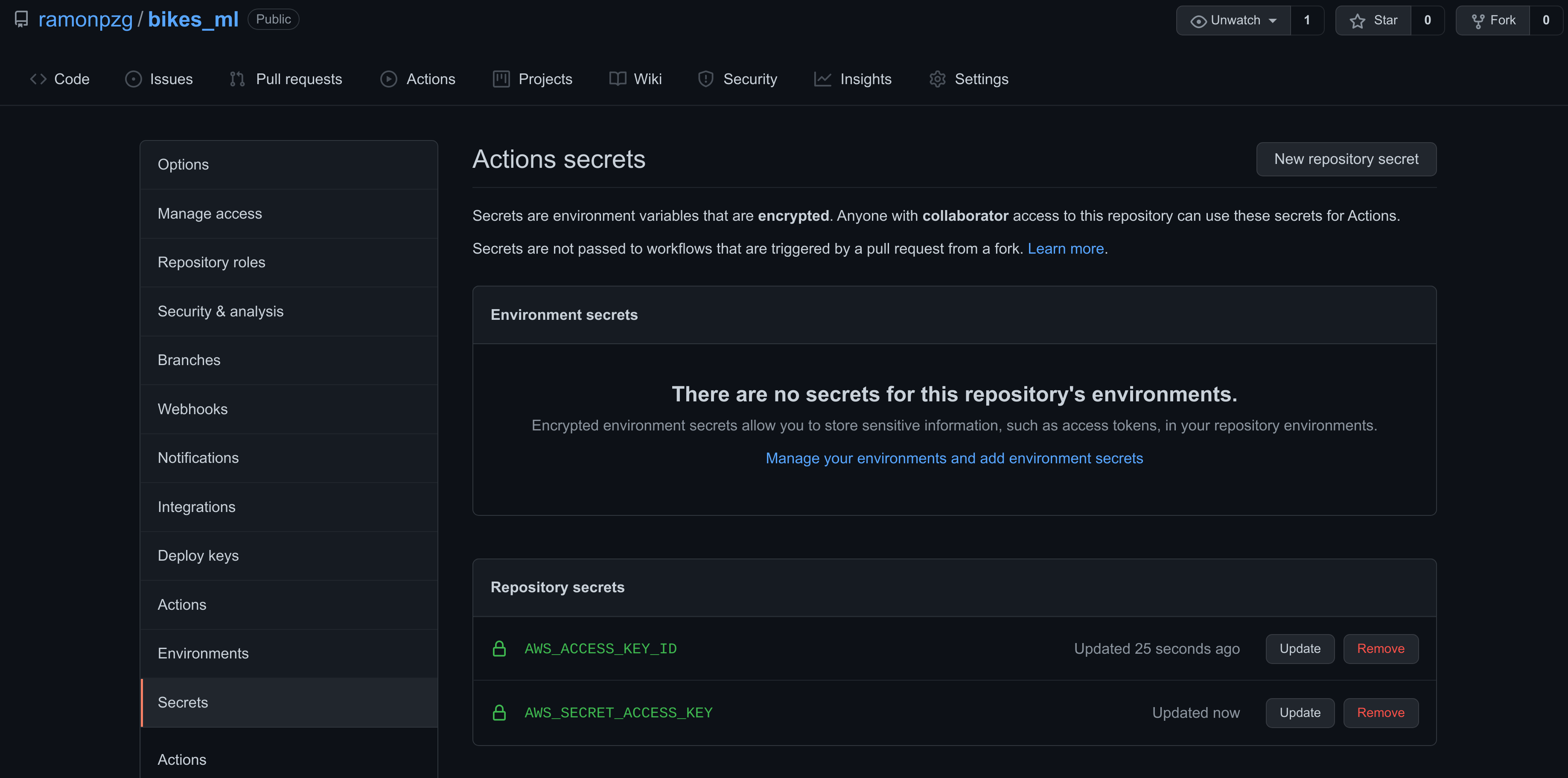
Add your AWS secrets to GitHub

1. Go to Settings > Secrets and click on New repository secret
2. On the Name box write AWS_ACCESS_KEY_ID
3. On the Value box write the access key you created earlier
4. Do the same as above for your AWS_SECRET_ACCESS_KEY

Once you finish adding them, it should look as follows.

Let’s add the yaml file from above to our special directory.

%%writefile .github/workflows/cml.yaml

name: bikes-pipeline-test
on: push
jobs:
  run:
    runs-on: [ubuntu-latest]
    container: docker://dvcorg/cml:0-dvc2-base1
    steps:
      - uses: actions/checkout@v2
      - name: cml_run 
        env:
          REPO_TOKEN: $
          AWS_ACCESS_KEY_ID: $
          AWS_SECRET_ACCESS_KEY: $
        run: |
          pip install -r requirements.txt

          dvc repro
          dvc push
          git fetch --prune

          echo "# CML Report" > report.md
          dvc metrics diff --show-md master >> report.md
          cml-send-comment report.md

!git status

%%bash

git add .
git commit -m "Adding CML CI/CD Pipeline"
git push

Immediately after commiting our changes with the cell above,

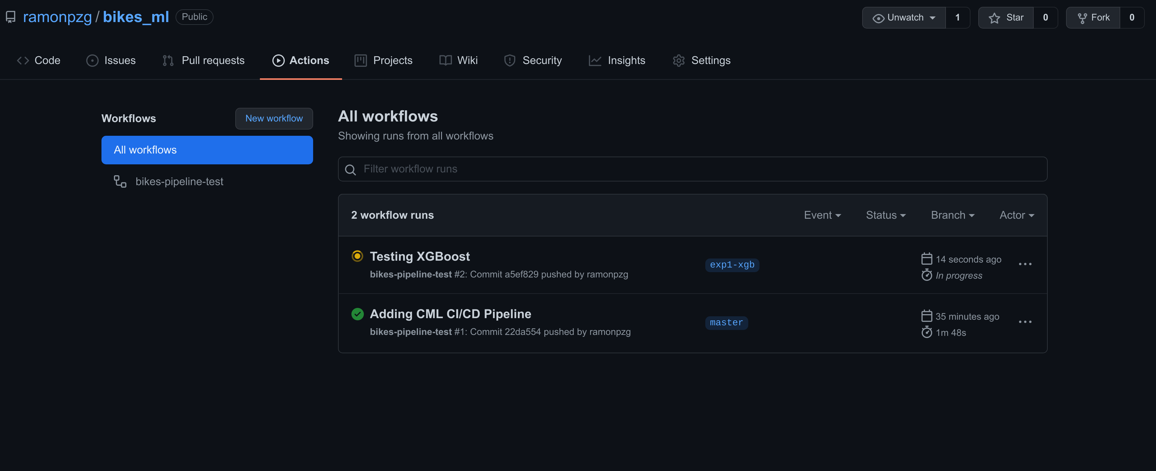
1. Navigate to the Actions tab
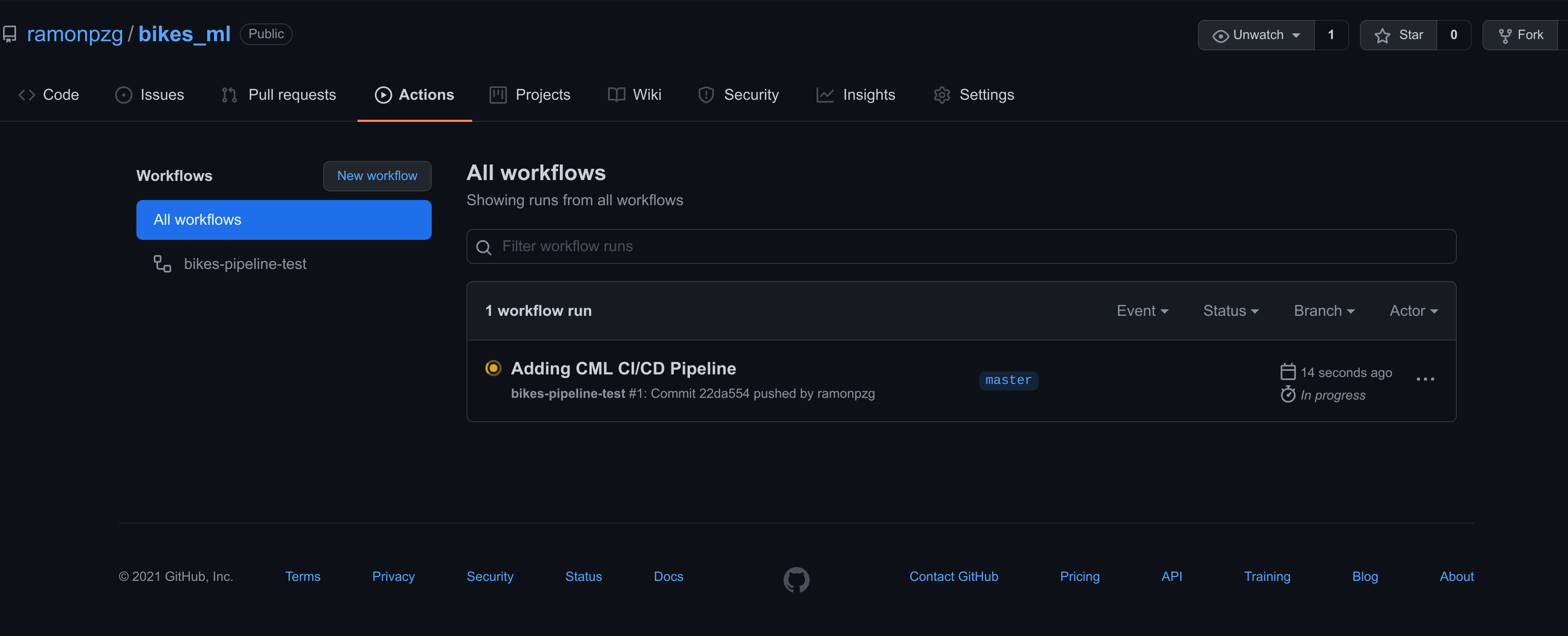
2. Click on Adding CML CI/CD Pipeline
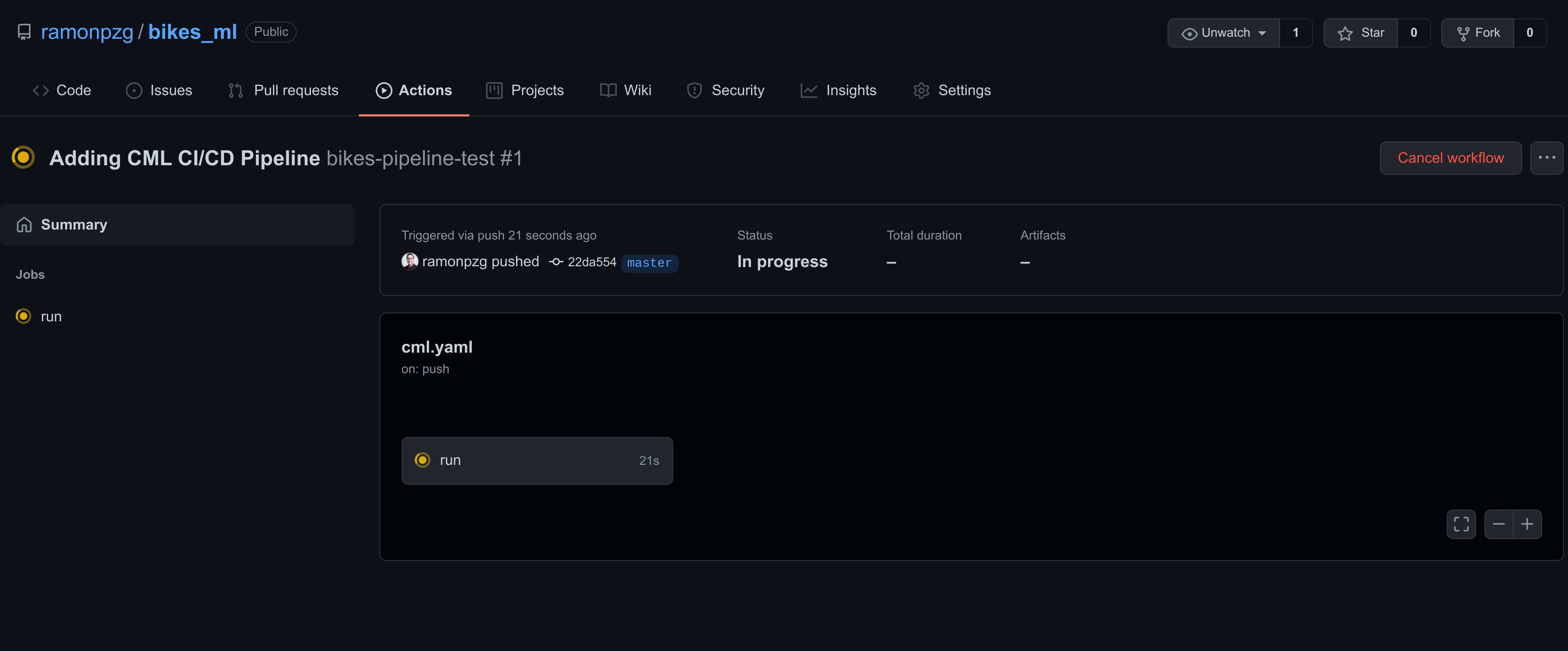
3. Click on run
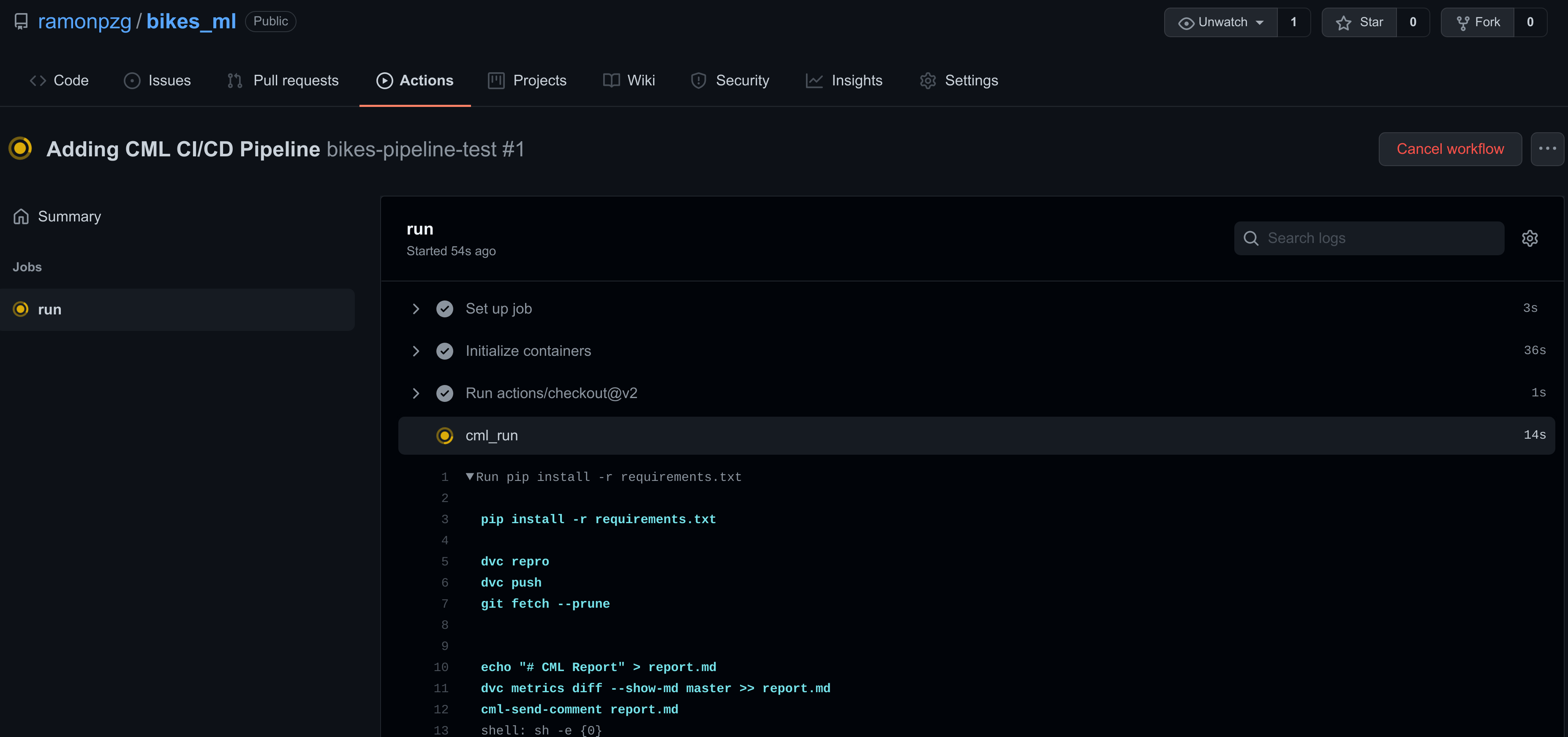
4. Once the yellow mark turns green and all of the steps in your run passed
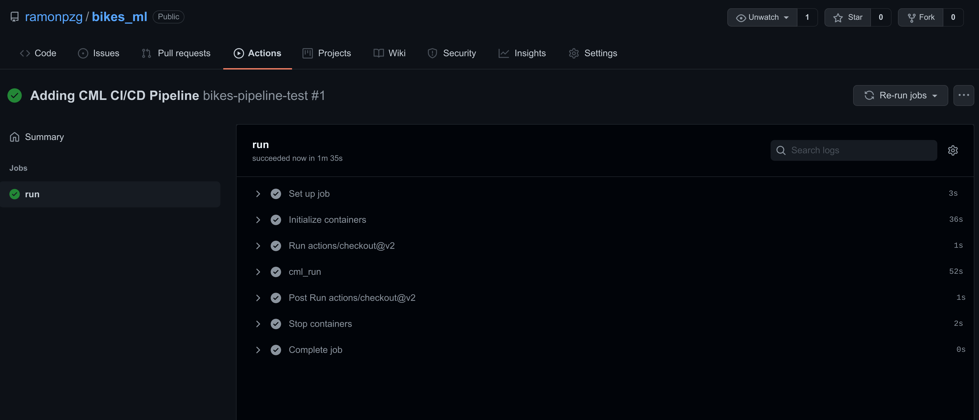
5. Go to your email and check out the results of your ML model
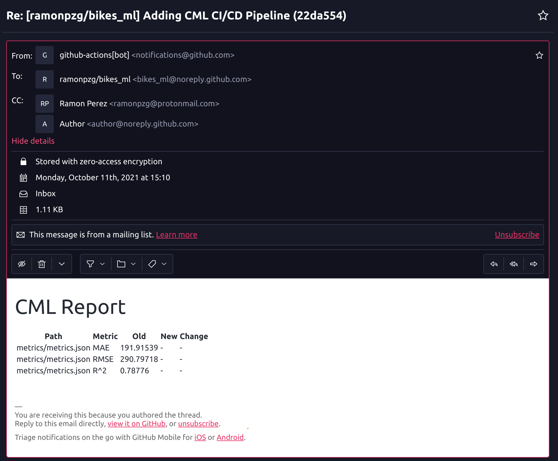
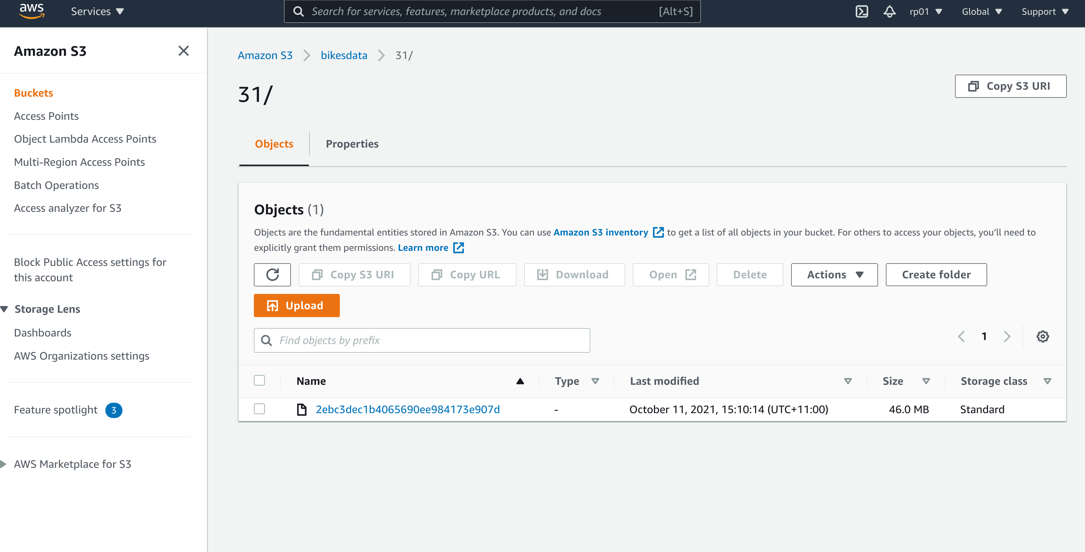
6. Then, check out the result in your bucket

Now that we have a system that will trigger a model training run with every change we make to our code, let’s go ahead and have some fun by testing other frameworks.

9. Experiments

We’ve been working inside our master branch using scikit-learn, and now we want to start experimenting with other tree-based frameworks like XGBoost, LightGBM, and CatBoost using different branches for each experiment. Let’s do just that and start by checking out a new branch, adding XGBoost to our train file, and triggering a new run.

!git checkout -b "exp1-xgb"

%%writefile src/train.py

import os, pickle, sys, pandas as pd
from xgboost import XGBRFRegressor

input_data = sys.argv[1]
output = os.path.join('models', 'rf_model.pkl')
seed, n_est = 42, 100

X_train = pd.read_csv(input_data)
y_train = X_train.pop('rented_bike_count')

rf = XGBRFRegressor(n_estimators=n_est, seed=seed)
rf.fit(X_train.values, y_train.values)

with open(output, "wb") as fd: pickle.dump(rf, fd)

Note that in order for GitHub to now we have been working in a different branch, we need to use the git push --set-upstream origin exp1-xgb command. Otherwise, we’ll get an error.

%%bash

git add .
git commit -m "Testing XGBoost"
git push --set-upstream origin exp1-xgb
git push

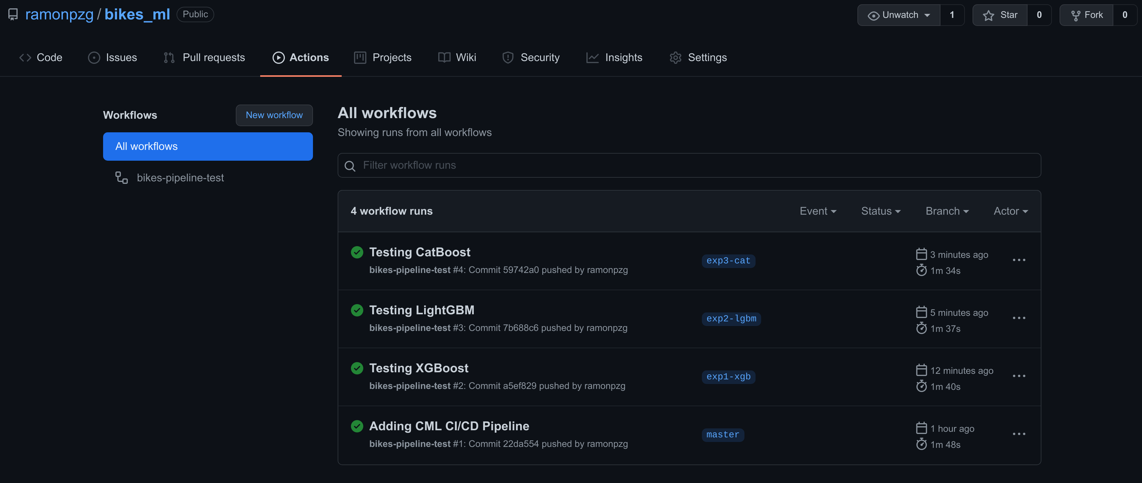
Following the same process as the one from the previous section, we can go to the Actions tab and have a look at our XGBoost run.

In addition, thanks to the dvc metrics diff --show-md master command in our CI/CD pipeline, we can now look at the difference in metrics between our current branch and the master one.

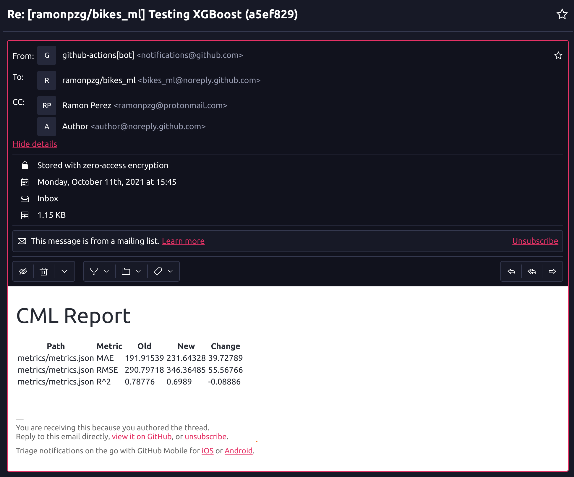
It seems that a plain baseline XGB model performs a bit worse than our sklearn one. Let’s try LightGBM and see how it does. We’ll move to a new branch, update the train.py file, and trigger the run on git push.

!git checkout -b "exp2-lgbm"

%%writefile src/train.py

import os, pickle, sys, pandas as pd
from lightgbm import LGBMRegressor

input_data = sys.argv[1]
output = os.path.join('models', 'rf_model.pkl')
seed, n_est = 42, 100

X_train = pd.read_csv(input_data)
y_train = X_train.pop('rented_bike_count')

rf = LGBMRegressor(n_estimators=n_est, random_state=seed)
rf.fit(X_train.values, y_train.values)

with open(output, "wb") as fd: pickle.dump(rf, fd)

%%bash

git add .
git commit -m "Testing LightGBM"
git push --set-upstream origin exp2-lgbm
git push

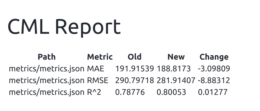The base implementation of LightGBM seems to have performed quite well. Let’s try out CatBoost now.

!git checkout -b "exp3-cat"

%%writefile src/train.py

import os, pickle, sys, pandas as pd
from catboost import CatBoostRegressor

input_data = sys.argv[1]
output = os.path.join('models', 'rf_model.pkl')
seed, n_est = 42, 100

X_train = pd.read_csv(input_data)
y_train = X_train.pop('rented_bike_count')

rf = CatBoostRegressor(n_estimators=n_est, random_state=seed)
rf.fit(X_train.values, y_train.values)

with open(output, "wb") as fd: pickle.dump(rf, fd)

%%bash

git add .
git commit -m "Testing CatBoost"
git push --set-upstream origin exp3-cat
git push

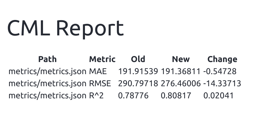
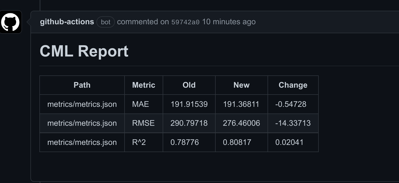
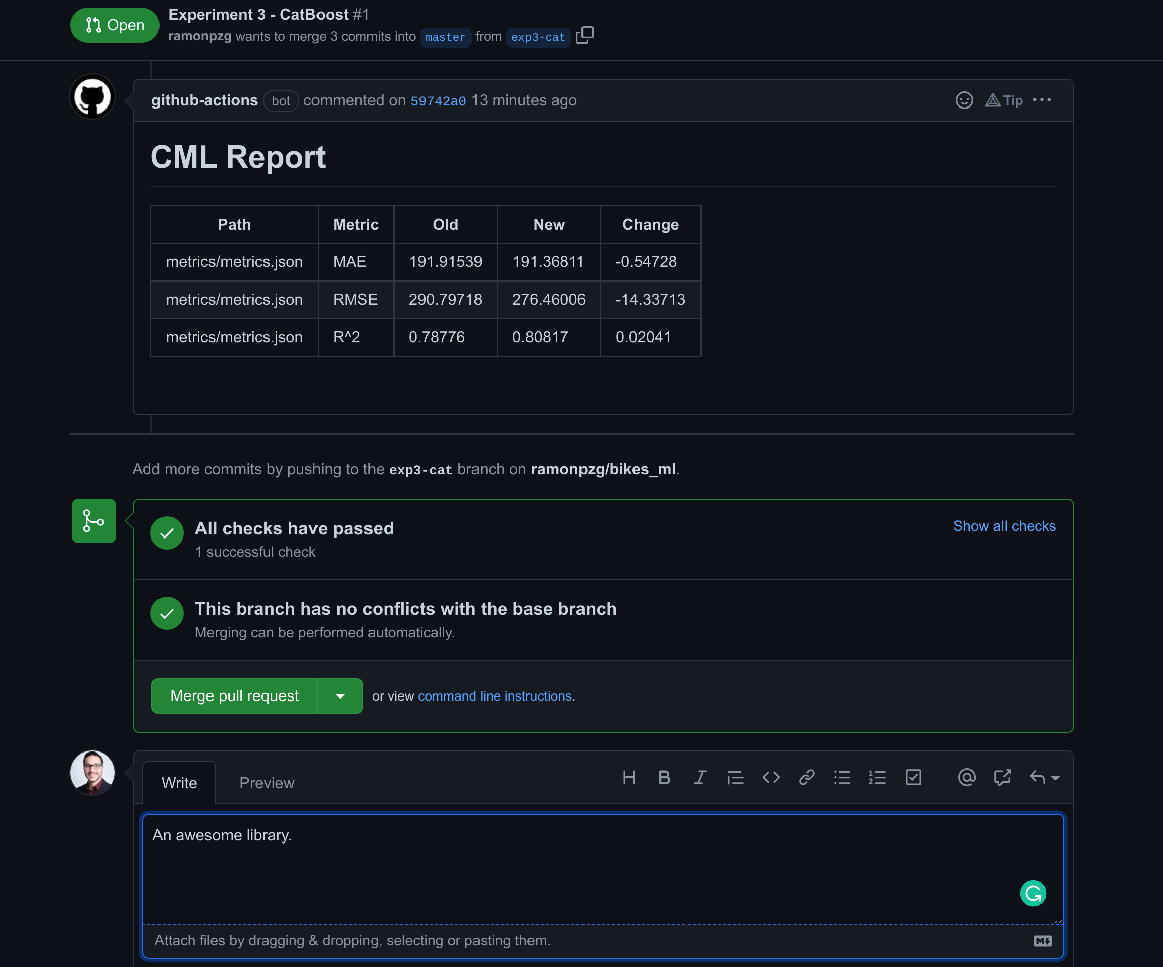
Surprisingly, CatBoost’s MAE performed a bit worse than LightGBM but RMSE performed much better.

You can go to your Actions tab again and see a recap of all of your runs.

We have a good candidate with CatBoost and we should merge this branch with master and start tunning our model.

10. Merging our Changes - PRs

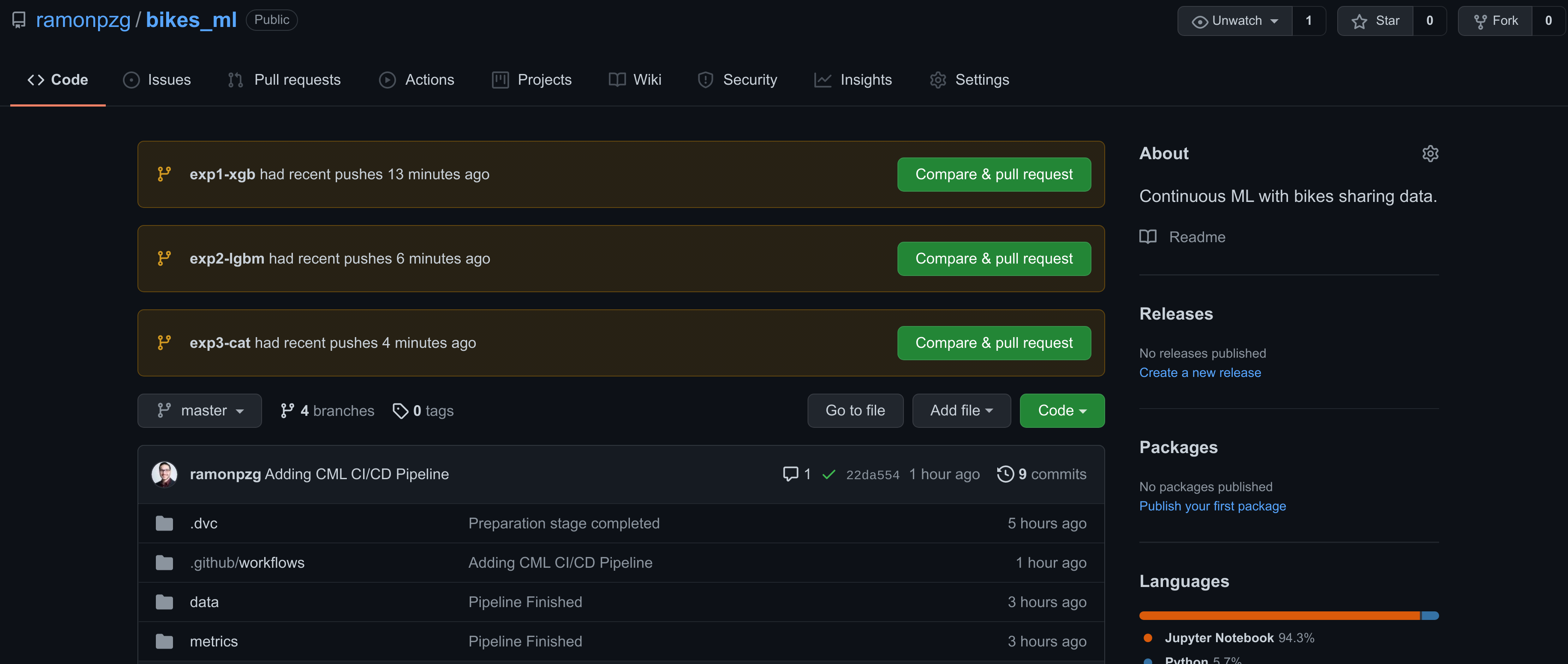If you go back to the main page of our repo, you’ll notice that GitHub has added a Compare & pull request option for each the three experiments. This is a nice shortcut to help us pick the one we liked best and add it to our main project’s branch, master.

So what is a pull request anyways? “A PR provides a user-friendly web interface for discussing proposed changes before integrating them into the official project.” ~ Atlassian

Let’s merge our experiment branch with our master branch.

1. Click on the Compare & pull request for exp3-cat.
2. Compare the changes.
3. Check out the report again.
4. Open a pull request with your details on why it should go to master.
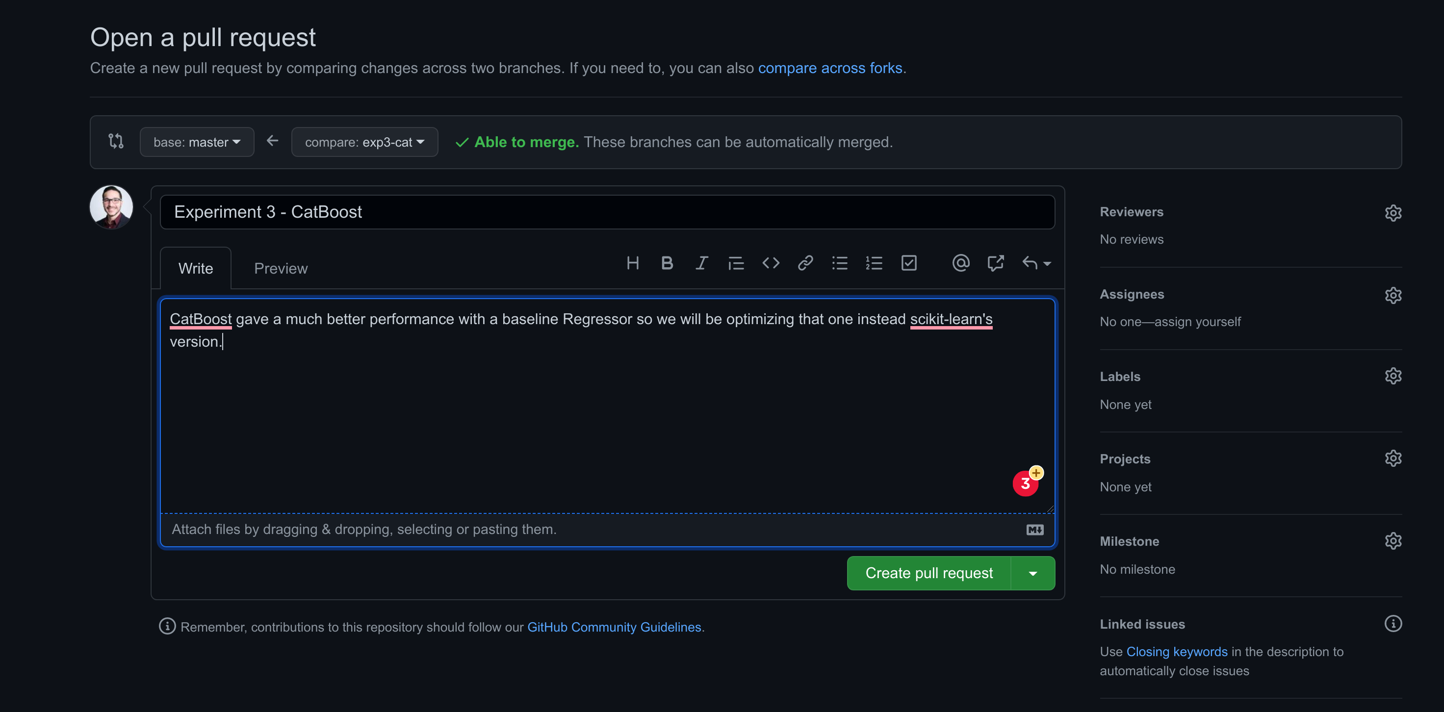
5. Once reviewed, write a comment and merge the pull request.
6. Lastly, we need to make sure our local env is up to date and once it is, we can switch to the master branch and work from there again. Run a git pull and a dvc pull.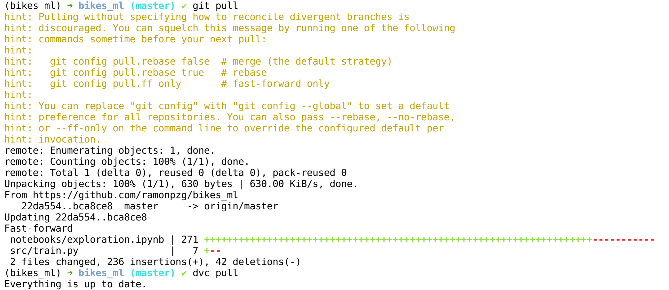

%%bash

git pull
dvc pull

11. Summary

Your project structure should now look similar to the following one.

.
├── data
│   ├── processed
│   │   ├── test.csv
│   │   └── train.csv
│   └── raw
│       └── SeoulBikeData.csv
├── dvc.lock
├── dvc.yaml
├── metrics
│   └── metrics.json
├── models
│   └── rf_model.pkl
├── new_user_credentials.csv
├── notebooks
│   └── exploration.ipynb
├── README.md
├── requirements.txt
├── src
│   ├── evaluate.py
│   ├── get_data.py
│   ├── prepare.py
│   └── train.py
└── tree_view.md

7 directories, 16 files

As you have seen throughout the tutorial, DVC helps us track our data, models, and metrics, and it also allows us to create pipelines for getting, preparing, and modeling data. In contrast, CML allows us to continuously deliver ML models through its CI/CD configuration alongside dvc. CML makes it easier to experiment and deploy models in a production environment.

DVC and CML are making possible what git alone can’t do for the machine learning community, and the do this by enhancing git in the parts where it’s lacking. Both tools should be in every data scientist and ML Engineer’s toolkit. Enough said!

12. Blind Spots and Future Work

Blind Spots

• We could have fine tuned our base model even further and make better comparisons with the other frameworks.
• We could have conducted more feature engineering.
• We could have selected the best features only based on feature importance.
• We could have done a bit more analysis of the data.
• We could have taken out the second dummy or our categorical variables. For example, there is no need to have Holiday and No Holiday as variables in our dataset.

Future Work

• If the data will be provided in the same formate we received it, then we need an easier transformation pipeline for the date, column names, and dummies.
• We could add the analytical tool, e.g. our dashboard, to the master branch and work with the models solely through branches.

13. Resources

Here are a few additional resources to dive deeped into some of the tools discussed above.

• DVC Get Started
• DVC Use Cases
• CML Get Started
• CatBoost Tutorial
• Git
• Pull Requests